Optimize Data lake layout using Clustering in Apache Hudi
Background
Apache Hudi brings stream processing to big data, providing fresh data while being an order of magnitude efficient over traditional batch processing. In a data lake/warehouse, one of the key trade-offs is between ingestion speed and query performance. Data ingestion typically prefers small files to improve parallelism and make data available to queries as soon as possible. However, query performance degrades poorly with a lot of small files. Also, during ingestion, data is typically co-located based on arrival time. However, the query engines perform better when the data frequently queried is co-located together. In most architectures each of these systems tend to add optimizations independently to improve performance which hits limitations due to un-optimized data layouts. This blog introduces a new kind of table service called clustering [RFC-19] to reorganize data for improved query performance without compromising on ingestion speed.
Clustering Architecture
At a high level, Hudi provides different operations such as insert/upsert/bulk_insert through it’s write client API to be able to write data to a Hudi table. To be able to choose a trade-off between file size and ingestion speed, Hudi provides a knob hoodie.parquet.small.file.limit to be able to configure the smallest allowable file size. Users are able to configure the small file soft limit to 0 to force new data to go into a new set of filegroups or set it to a higher value to ensure new data gets “padded” to existing files until it meets that limit that adds to ingestion latencies.
To be able to support an architecture that allows for fast ingestion without compromising query performance, we have introduced a ‘clustering’ service to rewrite the data to optimize Hudi data lake file layout.
Clustering table service can run asynchronously or synchronously adding a new action type called “REPLACE”, that will mark the clustering action in the Hudi metadata timeline.
Overall, there are 2 parts to clustering
- Scheduling clustering: Create a clustering plan using a pluggable clustering strategy.
- Execute clustering: Process the plan using an execution strategy to create new files and replace old files.
Scheduling clustering
Following steps are followed to schedule clustering.
- Identify files that are eligible for clustering: Depending on the clustering strategy chosen, the scheduling logic will identify the files eligible for clustering.
- Group files that are eligible for clustering based on specific criteria. Each group is expected to have data size in multiples of ‘targetFileSize’. Grouping is done as part of ‘strategy’ defined in the plan. Additionally, there is an option to put a cap on group size to improve parallelism and avoid shuffling large amounts of data.
- Finally, the clustering plan is saved to the timeline in an avro metadata format.
Running clustering
- Read the clustering plan and get the ‘clusteringGroups’ that mark the file groups that need to be clustered.
- For each group, we instantiate appropriate strategy class with strategyParams (example: sortColumns) and apply that strategy to rewrite the data.
- Create a “REPLACE” commit and update the metadata in HoodieReplaceCommitMetadata.
Clustering Service builds on Hudi’s MVCC based design to allow for writers to continue to insert new data while clustering action runs in the background to reformat data layout, ensuring snapshot isolation between concurrent readers and writers.
NOTE: Clustering can only be scheduled for tables / partitions not receiving any concurrent updates. In the future, concurrent updates use-case will be supported as well.
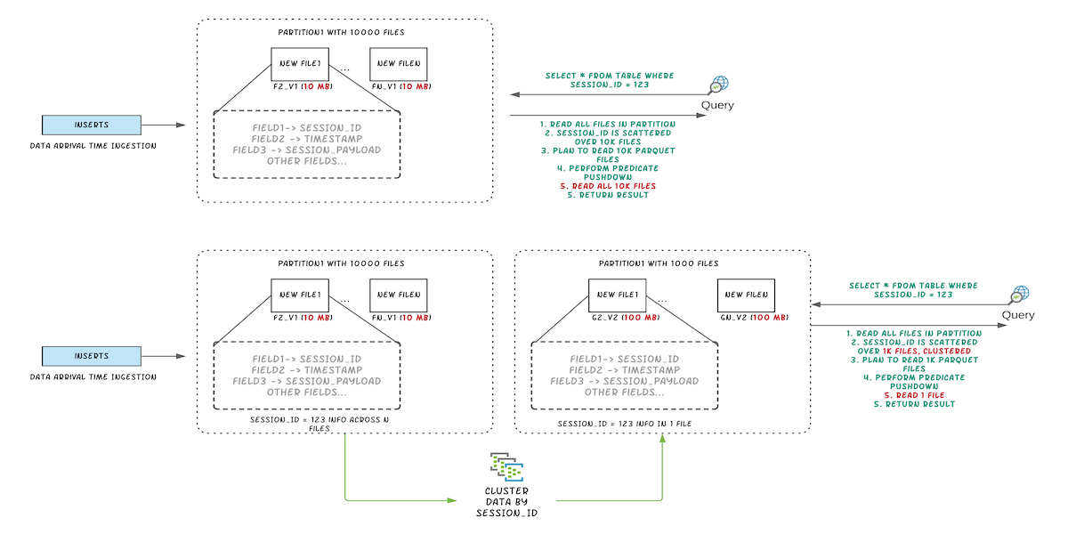 Figure: Illustrating query performance improvements by clustering
Setting up clustering
Inline clustering can be setup easily using spark dataframe options. See sample below
import org.apache.hudi.QuickstartUtils._
import scala.collection.JavaConversions._
import org.apache.spark.sql.SaveMode._
import org.apache.hudi.DataSourceReadOptions._
import org.apache.hudi.DataSourceWriteOptions._
import org.apache.hudi.config.HoodieWriteConfig._


val df =  //generate data frame
df.write.format("org.apache.hudi").
        options(getQuickstartWriteConfigs).
        option(PRECOMBINE_FIELD_OPT_KEY, "ts").
        option(RECORDKEY_FIELD_OPT_KEY, "uuid").
        option(PARTITIONPATH_FIELD_OPT_KEY, "partitionpath").
        option(TABLE_NAME, "tableName").
        option("hoodie.parquet.small.file.limit", "0").
        option("hoodie.clustering.inline", "true").
        option("hoodie.clustering.inline.max.commits", "4").
        option("hoodie.clustering.plan.strategy.target.file.max.bytes", "1073741824").
        option("hoodie.clustering.plan.strategy.small.file.limit", "629145600").
        option("hoodie.clustering.plan.strategy.sort.columns", "column1,column2"). //optional, if sorting is needed as part of rewriting data
        mode(Append).
        save("dfs://location");
For more advanced usecases, async clustering pipeline can also be setup. See an example here.
Table Query Performance
We created a dataset from one partition of a known production style table with ~20M records and on-disk size of ~200GB. The dataset has rows for multiple “sessions”. Users always query this data using a predicate on session. Data for a single session is spread across multiple data files because ingestion groups data based on arrival time. The below experiment shows that by clustering on session, we are able to improve the data locality and reduce query execution time by more than 50%.
Query:
spark.sql("select * from table where session_id=123")
Before Clustering
Query took 2.2 minutes to complete. Note that the number of output rows in the “scan parquet” part of the query plan includes all 20M rows in the table.
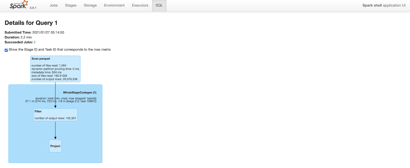 Figure: Spark SQL query details before clustering
After Clustering
The query plan is similar to above. But, because of improved data locality and predicate push down, spark is able to prune a lot of rows. After clustering, the same query only outputs 110K rows (out of 20M rows) while scanning parquet files. This cuts query time to less than a minute from 2.2 minutes.
 Figure: Spark SQL query details after clustering
The table below summarizes query performance improvements from experiments run using Spark3
| Table State | Query runtime | Num Records Processed | Num files on disk | Size of each file |
|---|---|---|---|---|
| Unclustered | 130,673 ms | ~20M | 13642 | ~150 MB |
| Clustered | 55,963 ms | ~110K | 294 | ~600 MB |
Query runtime is reduced by 60% after clustering. Similar results were observed on other sample datasets. See example query plans and more details at the RFC-19 performance evaluation.
We expect dramatic speedup for large tables, where the query runtime is almost entirely dominated by actual I/O and not query planning, unlike the example above.
Summary
Using clustering, we can improve query performance by
- Leveraging concepts such as space filling curves to adapt data lake layout and reduce the amount of data read during queries.
- Stitch small files into larger ones and reduce the total number of files that need to be scanned by the query engine.
Clustering also enables stream processing over big data. Ingestion can write small files to satisfy latency requirements of stream processing. Clustering can be used in the background to stitch these small files into larger files and reduce file count.
Besides this, the clustering framework also provides the flexibility to asynchronously rewrite data based on specific requirements. We foresee many other use-cases adopting clustering framework with custom pluggable strategies to satisfy on-demand data lake management activities. Some such notable use-cases that are actively being solved using clustering:
- Rewrite data and encrypt data at rest.
- Prune unused columns from tables and reduce storage footprint.